
There are many powerful tools like Keras and Tensorflow out there to make convolutional neural networks (CNNs). However, unless I have opened the hood and peeked inside, I am not really satisfied that I know something. If you are like me read on to see how to build CNNs from scratch using Numpy (and Scipy).
The code for this post is available in my repository
There are many powerful tools like Keras and Tensorflow out there to make convolutional neural networks (CNNs). However, unless I have opened the hood and peeked inside, I am not really satisfied that I know something. If you are like me read on to see how to build CNNs from scratch using Numpy (and Scipy).
I am making this post a multi part post. As of now I have planned two parts. In the first I will only do a two class classification problem on Fashion MNIST restricted to two classes. The images are monochromatic and the CNN will have only one convolutional filter followed by a dense layer. This simplicity will allow us to focus on the details of convolution without worrying about incidental complexity. In the second post I will tackle the full Fashion MNIST dataset (10 classes) and multiple convolution filters. I will also look at the CIFAR-10 dataset which has colored images in 10 classes.
This is going to a technical post and certain familiarity with algebra and calculus is assumed. While I know that one can do a lot with tensorflow without knowing advanced math, I do not see how it is possible to peek under the hood without the same. Algebra is essential in the forward pass and algebra and calculus are useful to compute the derivative of the loss function with respect to the weights of the network which I derive in closed form. These are used to update the weights, something commonly known as back propagation. Readers unwilling to go through the derivation but able to follow the final expressions can still benefit by understanding the final results and implementing (or following my implementation) in numpy.
Convolution
In this section we will discuss what exactly we mean by convolution in image processing and how it is related to the implementation in scipy. This is useful as scipy implementation is much faster than a naive numpy implementation. In the end we will consider an example where we compute the convolution by hand and by using scipy as a sanity check. For simplicity we will work in 1 dimension for this section but the arguments extend simply to any number of dimensions.
Mathematically a convolution of a function f by a function g is defined as
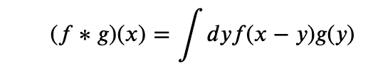
This definition is useful in physics and signal processing. For instance in electromagnetism g could be the charge density and f (called a Green’s function in that case) would help us compute the potential due to said charge distribution. (See books on electromagnetism like Jackson or particle physics like Peskin and Schroeder for more details).
In image processing this definition is a bit backwards in that for a convolution window g , of length , we would want the convolution at to be the weighted average of such that the value at −/2+ is weighted by (). Thus, for image processing purposes the correct definition is
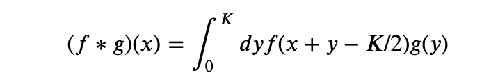
Note that this will require value of f(x) for negative values of x and if this is put in as it is then numpy will interpret the negative numbers as indexing from the end of the array. Thus, while implementing this in numpy, we need to make sure that the original array is embedded in a bigger 0-padded one and negative indexes are understood appropriately.
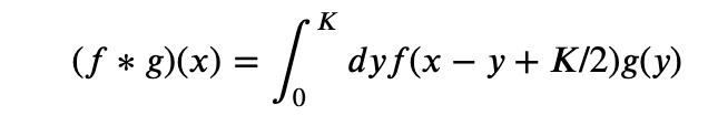
In our implementation of CNNs, we will use scipy.convolve as it will be faster than a naive implementation in numpy. So it is useful to understand the way scipy.convolve is related to what we want. Scipy’s convolve is for signal processing so it resembles the conventional physics definition but because of numpy convention of starting an array location as 0, the center of the window of g is not at 0 but at K/2. So scipy.convolve uses the definition
Now, we if reverse the scipy convolution window we have y ->K-y and that makes the integral
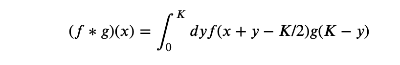
Thus we will get the result we want by giving the reversed array of the convolution window to scipy.convolve.
As an example consider the signal and filter given below.
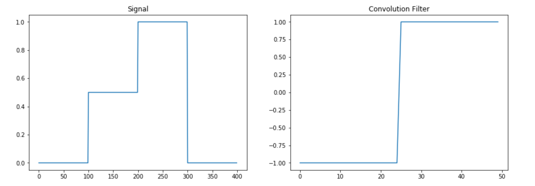
We then implement the convolution by hand and using scipy in the following command
convolve(sig,win[::-1],'same')
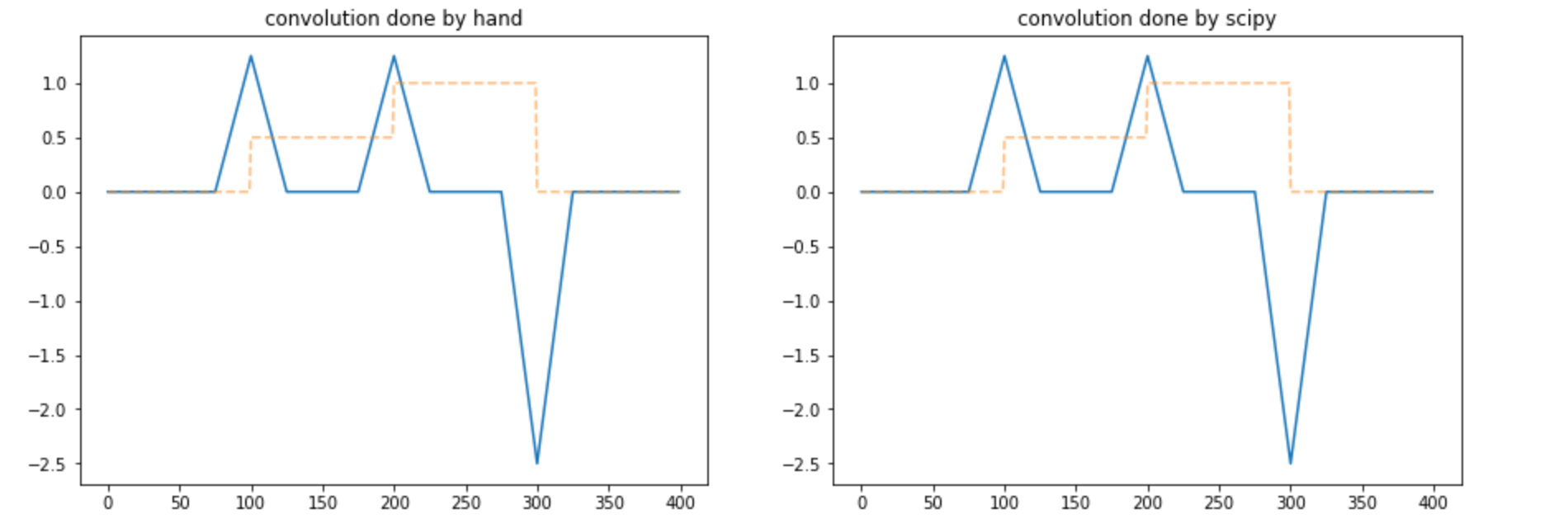
The results are plotted below. The reader is advised to convince herself that the results are the same either by eyeballing the graphs or implementing the two methods herself.
We are now ready to implement CNNs using numpy.
Two-class classification
As our first example we implement a two class classification using numpy. I discuss this in full detail and for the other examples in latter posts I will expect that the reader has understood this example in detail and go a bit faster.
For the data we will used the Fashion MNIST. We get this from Keras as it is easily available but do note that this is the only use of Keras in this post.
(X_train_full, y_train_full), (X_test, y_test) = keras.datasets.fashion_mnist.load_data()
We then restrict our dataset to just the category 1 and 3.
cond=np.any([y_train_full==1,y_train_full==3],0)X_train_full=X_train_full[cond]
y_train_full=y_train_full[cond]
X_test=X_test[np.any([y_test==1,y_test==3],0)]
y_test=y_test[np.any([y_test==1,y_test==3],0)]y_train_full=(y_train_full==3).astype(int)
y_test=(y_test==3).astype(int)
We then split our training set into a train and validation set
X_train, X_valid = X_train_full[:-1000], X_train_full[-1000:]
y_train, y_valid = y_train_full[:-1000], y_train_full[-1000:]
And we finally standardize the data as Neural Networks work best with data with vanishing mean and unit standard deviation.
X_mean = X_train.mean(axis=0, keepdims=True)
X_std = X_train.std(axis=0, keepdims=True) + 1e-7
X_train = (X_train - X_mean) / X_std
X_valid = (X_valid - X_mean) / X_std
X_test = (X_test - X_mean) / X_std
Our data are monochrome images that come as matrices of dimension L x L (here L=28). For simplicity we have only one convolution layer (we will relax this restriction in later posts) which is a matrix of size K x K (we will take K=3 in our examples) whose weights can be learnt. In addition we have a dense layer which is a matrix of size (L*L) x 1. Note that we have not kept bias terms and the reader can include them as an exercise once she has understood this example.
We now describe the forward pass, the error and the back propagation in some detail.
Forward Pass
- We get the images and refer to it as the 0-th layer 0
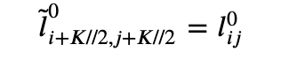
- We embed the image centered into one of size (+,+) with zero padding
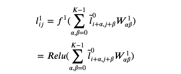
- Then we pass it through a convolutional layer and an activation function f1 (that we will take to be Relu). This is the first layer l1.
- Finally we make a dense layer wrapped in a function f2 (which in this case we take to be a sigmoid function). This is the second layer l2.
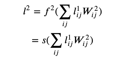
Note that even though the weights W2 are for a dense layer we have written the indices here without flattening as it has an intuitive interpretation in that it takes each pixel of the convoluted image and makes a weighted sum. Nevertheless, flattening both and doing a numpy dot is more performant and that is what we do in the code below.
The Loss Function
For the loss function we take the usual log-loss
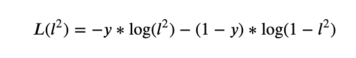
where y is the true outcome.
Backpropagation
Backpropagation is just a fancy word for saying that all the learnable weights are corrected by the gradient of the loss function with respect to the weights that are being learned. It is straightforward to differentiate the loss function with respect to W1 and W2 using the chain rule.
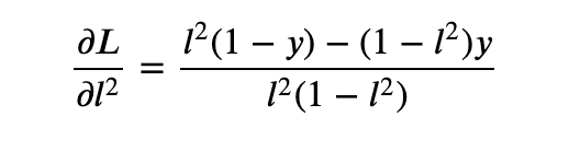
- The derivative of the loss function with respect to the layer 2 is
- The derivative of the loss function with respect to the dense layer weights is
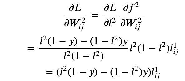
where we have used the fact that l2 is the output of the sigmoid function s(x) and that s’(x)=s(x)(1-s(x)).
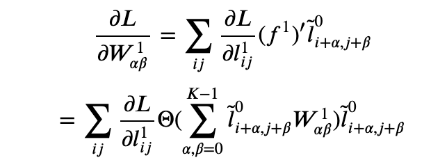
- Similarly, the derivative of the loss function with respect to layer 1 is
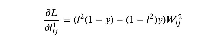
- The derivative of the loss function with respect to the convolution filter is
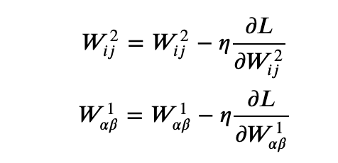
Now we have closed form expressions for the derivative of the loss function with respect to the weights of the convolution filter as well as the final dense matrix so we can update the weights (with a hyperparameter the learning rate) as
That’s it.
That is all that is required to write the implementation of the CNN. Before doing that we first note the loss function and accuracy for initial random weights so as to have a benchmark.
Loss and accuracy before training
Before training starts, the loss on average can be obtained analytically from the expression for the loss and is 1. The accuracy is 0.5. We will run our code over five epochs and see the loss and accuracy on the test and validation set.
The code
First we write some custom functions for Relu, its derivative and the sigmoid function that we require for the main code and a function to just do the forward pass and compute loss and accuracy to do so on the validation set
def relu(x):
    return np.where(x>0,x,0)

def relu_prime(x):
    return np.where(x>0,1,0)

def sigmoid(x):
    return 1./(1.+np.exp(-x))

def forward_pass(W1,W2,X,y):
    l0=X
    l0_conv=convolve(l0,W1[::-1,::-1],'same','direct')

    l1=relu(l0_conv)
    l2=sigmoid(np.dot(l1.reshape(-1,),W2))
    l2=l2.clip(10**-16,1-10**-16)
    loss=-(y*np.log(l2)+(1-y)*np.log(1-l2))
    accuracy=int(y==np.where(l2>0.5,1,0))
    return accuracy,loss
Now we write the main part of the code
# learning rate
eta=.001
for epoch in range(5):
    # custom code to keep track of quantities to
    # keep a running average. it is not shown for clarity.
    # the reader can implement her own or ask me in the comments.    train_loss, train accuracy=averager(), averager()

    for i in range(len(y_train)):

        # Take a random sample from train set
        k=np.random.randint(len(y_train))
        X=X_train[k]
        y=y_train[k]

        ##### FORWARD PASS ######

        # First layer is just the input
        l0=X

        # Embed the image in a bigger image.
        # It would be useful in computing corrections
        # to the convolution filter
        lt0=np.zeros((l0.shape[0]+K-1,l0.shape[1]+K-1))
        lt0[K//2:-K//2+1,K//2:-K//2+1]=l0

        # convolve with the filter
        # Layer one is Relu applied on the convolution                l0_conv=convolve(l0,W1[::-1,::-1],'same','direct')
        l1=relu(l0_conv)

        # Compute layer 2
        l2=sigmoid(np.dot(l1.reshape(-1,),W2))
        l2=l2.clip(10**-16,1-10**-16)

        ####### LOSS AND ACCURACY #######
        loss=-(y*np.log(l2)+(1-y)*np.log(1-l2))
        accuracy=int(y==np.where(l2>0.5,1,0))

        # Save the loss and accuracy to a running averager
        train_loss.send(loss)
        train_accuracy.send(accuracy)

        ##### BACKPROPAGATION #######

        # Derivative of loss wrt the dense layer
        dW2=(((1-y)*l2-y*(1-l2))*l1).reshape(-1,)

        # Derivative of loss wrt the output of the first layer
        dl1=(((1-y)*l2-y*(1-l2))*W2).reshape(28,28)

        # Derivative of the loss wrt the convolution filter        f1p=relu_prime(l0_conv)
        dl1_f1p=dl1*f1p
        dW1=np.array([[
           (lt0[alpha:+alpha+image_size,beta:beta+image_size]\
           *dl1_f1p).sum() for beta in range(K)]\
           for alpha in range(K)])

        W2+=-eta*dW2
        W1+=-eta*dW1
    loss_averager_valid=averager()
    accuracy_averager_valid=averager()

    for X,y in zip(X_valid,y_valid):
        accuracy,loss=forward_pass(W1,W2,X,y)
        loss_averager_valid.send(loss)
        accuracy_averager_valid.send(accuracy)

    train_loss,train_accuracy,valid_loss,valid_accuracy\
            =map(extract_averager_value,[train_loss,train_accuracy,
                 loss_averager_valid,accuracy_averager_valid])

    # code to print losses and accuracies suppressed for clarity
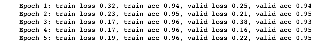
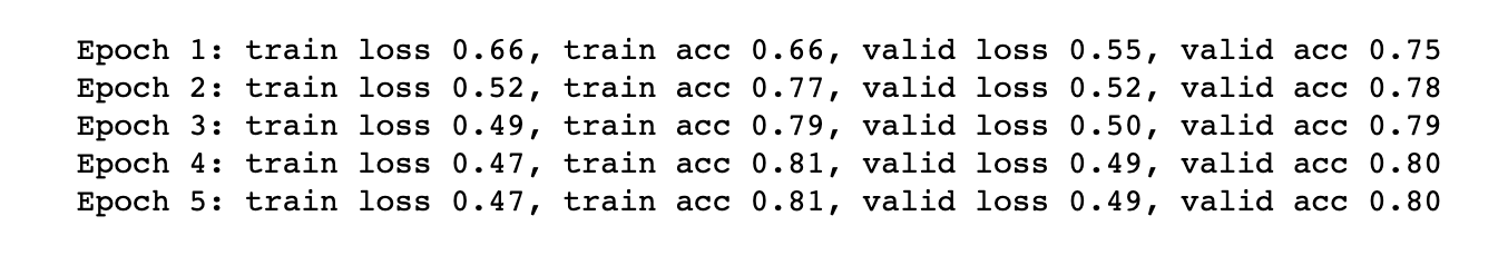
On my trial run I got the following results. Your’s should be similar
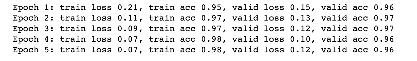
We can see that even this simple model reduces the loss from about 1 to 0.1 and increases the accuracy from 0.5 to about 0.96 (on the validation set).
We can visualize the convolution by plotting a few (standardized) images and their convolution with the original random filter and the final trained one.
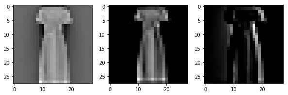
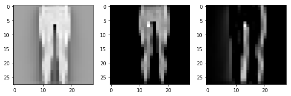
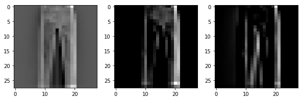
We see that the convolution filter seems to have learned to identify the right edges somewhat. It should be better when we train multiple filters but we have kept things simple by having just one filter. (This choice itself is a hyperparameter). We can do one more thing before finishing off part 1 of this post. We can make two more models: 1) We freeze the convolution layer weights and 2) We freeze the dense layer weights. This would help us understand if these layers contribute to the process. This is very easy. For the former we comment out the update line for W1
W2+=-eta*dW2
# W1+=-eta*dW1
and for the latter we comment out the update line for W2
# W2+=-eta*dW2
W1+=-eta*dW1
The resulting loss and accuracy are
and
respectively. It is clear that most of the work is done by the dense layer but we can still get a loss of .5 and an accuracy of .8 by just the convolution layer. Presumably this performance will increase with a larger number of filters. We will explore this in later posts.