Convolutional Neural Networks Using Numpy – Part 2

Motivation

This post is written to show an implementation of Convolutional Neural Networks (CNNs) using numpy. I have made a similar post earlier but that was more focused on explaining what convolution in general and CNNs in particular are whereas in this post the focus will also be more on implementing them efficiently in numpy by using vectorization.

It is worth pointing out that compared to packages like tensorflow, pytorch etc., using numpy does not offer any benefits in speed in general. In fact if one includes development time, it is most likely slower. The idea of the post is not to advertise the use of numpy for speed but to share the author’s experience of rebuilding the wheel. While the same is often derided, or demonized even, it is only with rebuilding a few wheels that one is able to to invent new machinery. Not to mention, sometime rebuilding the wheel is just plain fun!

We will focus solely on the CNN part of it and the other related aspects like activation function and maxpooling etc will not discussed here as they can be implemented as separate layers acting on the output of the CNN layer. However, we do discuss padding and stride which are inherent to the convolution process.

The code for this post can be found in the repository with most of the code contained in the file CNN.py

Since the goal of the post is to show how to make an efficient implementation of CNNs in numpy, I will not provide all the code in this post but instead explain the idea of what is being done with lots of visualization and only the relevant code. All the code can of course be found in the aforementioned repository.

Convolutional Neural Networks

Forward Pass

We will work on 2 dimensional images with multiple channels. For actual images the number of channels is either 1 for monochrome images or 3 (Red/Green/Blue or RGB in short) for colored images. However, a CNN could itself act on the output of a previous CNN and then the meaning of channels is the output of different filters of the previous layer and so the number of  channels can be any positive integer. Nevertheless, below we concretely talk about 3 channels while coloring them RGB to help visualize the process.

The convolution layer has the filter weights as learnable parameters and two hyperparameters – the stride and the padding. These are denoted below as
$$
W_{ijkl},s,p
$$
which are a 4 dimensional tensor and two scalars respectively.  The first two dimensions of the weights run over the row and column of the convolutional filter whereas the third one runs over the input channels and the fourth one over the output channels. Note that the the stride and padding can be different for each dimension of the image but for notational simplicity we keep them the same below (although in the actual code allows for different values).

We denote the input of a convolution layer by
$$
l^0_{I,i,j,k}
$$
where the indices are the minibatch, the row, the column and the channel respectively. The output is similarly denoted by
$$
l^1_{I,i,j,l}
$$
However, note that except for the minibatch index, the others may  have a different range than that of the input ones. This means that the output image sizes and number of channels may be different.

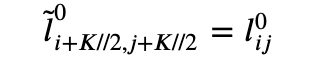
The notion of padding comes from embedding this image in a (possibly) bigger 0-padded array
$$
\tilde l^0_{I,P+i,P+j,k}=l^0_{I,i,j,k}
$$
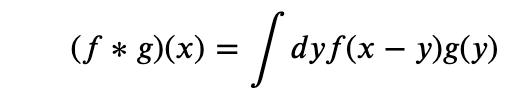
where \(P\) is the padding. The convolution operation is defined as
$$
l^1_{I,i,j,l} = \sum_{\alpha,\beta,k} \tilde l^0_{I,si+\alpha,sj+\beta,k} W_{\alpha,\beta,k,l}
$$
where \(s\) is the stride.

In order to understand the above, we visualize this process by taking an “image” of size \(6 \times 8\) with three channels where we fill in the values sequentially. So the red channel has its first row from 0 to 7, the second row from 8 to 15 and so on till the 6th row going up to 47. The green channel then starts from 48 and fills in the same way.


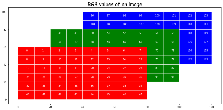
In the above we plot the channels along the depth direction.

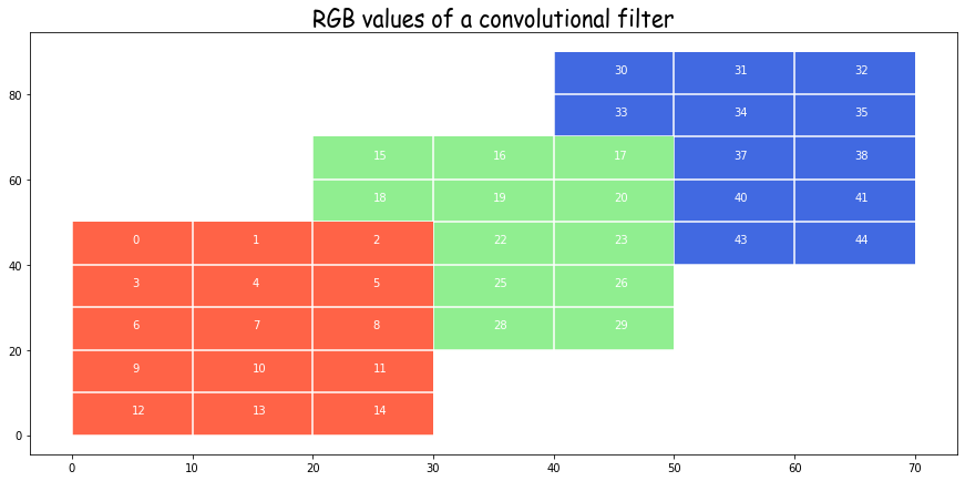
We make a “filter” as having the same structure but a different size. Specifically we take \(5 \times 3\) size filters. Note that while there are three filters here, one for each input channel, this set will produces just one channel of output. For each channel of the output we will need a separate copy of such three filters.

Now we  consider the effect of the red filter on the red channel.  Before doing that take another look at the expressions for convolutions from above and try to understand what is happening.

In the example in the image below we have taken a padding of 2 in the y-direction and 1 in the x-direction. This means the original image is embedded in the center of a 0-padded array of a bigger size by 4 in the y-direction and 2 in the x-direction. This ensures that the output of convolution is the same size as the input (in the absence of a stride) but we do not have to do that. Padding can be small or perversely bigger.

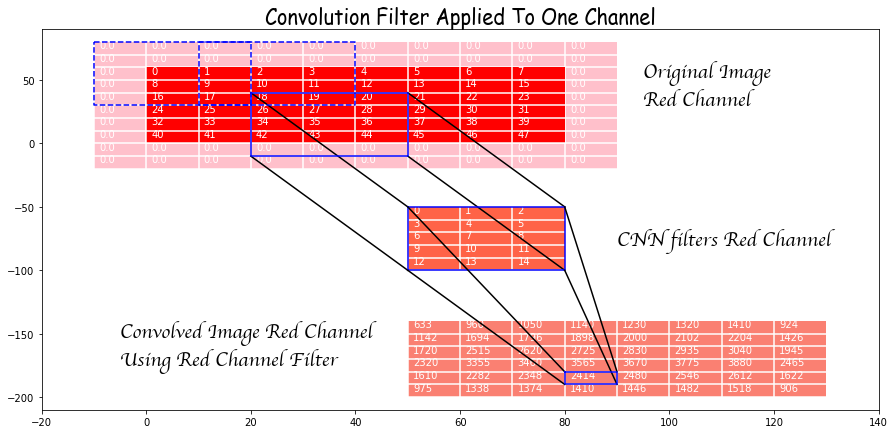
Now look at the effect of convolution of the red filter on the part of the (larger embedded) image in the box starting at (4,3) and of the same size as the filter that is drawn in solid blue. Each element of the window is multiplied by the corresponding element of the filter and the result is then summed. Note that this involves a row of zero-padded values. This sum is the (4,3) rd element of the convolution of the red channel. If we had not zero-paded we could not even have this entry and the output would be limited to those values that come from convolution filters fitting completely inside the original (non zero-padded) image.

Let’s also look at the stride. The effect of the stride can be seen from the theoretical expression. A stride of 1 is the default and its result is shown above. However, if we were to choose a stride of 2, for instance, then the windows used would be like the dashed-blue windows and we see that they are moved in steps of 2.

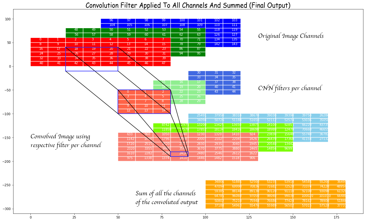
The final ouput of one filter of 3 channels is given by summing the convolution on the three channels as shown below.

Backpropagation

During backpropagation, the layer receives as input the derivative of the loss with respect to the forward pass output \(\frac{\partial L}{\partial l^1}\) and outputs the derivative of the loss with respect to the forward pass input \(\frac{\partial L}{\partial l^0}\) . If the weights are learnable then during backpropagation the layer also adjusts the weights according to the weight updation rule. For the purpose of weight updation, one needs the derivative of the loss with respect to the weights \( \frac{\partial L}{\partial W}\). (Note that we are implicitly considering only updates that depend on the first derivative of the loss but the discussion can be generalized in a straightforward way to update methods that use higher derivative to compute momentum etc.)

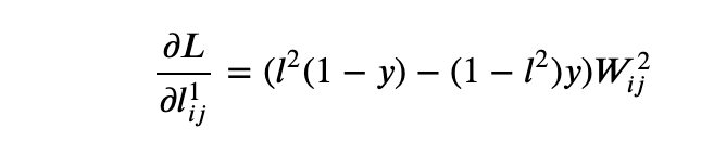
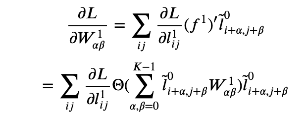
The derivative of the loss with respect to the weights is given by
$$
\frac{\partial L}{\partial W_{\alpha,\beta,k,m}}=\sum_{I,i,j} \frac{\partial L}{\partial l^1_{I,i,j,m}} \tilde l^0_{I,si+\alpha,sj+\beta,k}
$$
and the derivative of the loss with respect to the input is given by
$$
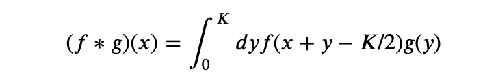
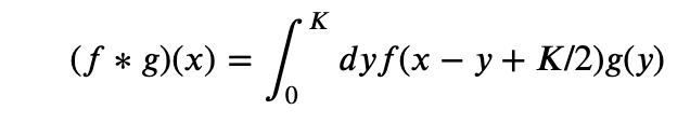
\frac{\partial L}{\partial l^0_{I,p,q,l}} = \sum_{\alpha,\beta,m} \left(\frac{\partial L}{\partial l^1} \right)_{I,\frac{p+P-\alpha}{s} , \frac{q+P-\beta}{s},m} W_{\alpha,\beta,l,m} \\
= \sum_{\alpha,\beta,m} \left(\frac{\partial L}{\partial l^1} \right)_{I,\frac{p+P-K+1+\alpha}{s} , \frac{q+P-K+1+\beta}{s},m} \tilde W_{\alpha,\beta,m,l}
$$
where
$$
\tilde W_{\alpha,\beta,m,l} = W_{K-\alpha, K-\beta,l,m}
$$

and \(K\) is the filter size. All these can be computed using simple algebra and the chain rule of calculus.

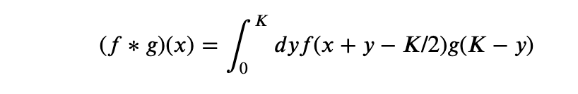
We observe that  the derivative of the loss with respect to the input layer is just a convolution of the error with respect to \(\frac{\partial L}{\partial l^1}\) with a filter that has the indices along the first two directions reversed.

This observation tells us that we can reuse our code for convolution but we still need to massage the data \(\frac{\partial L}{\partial l^1}\) before we do that. We can first embed the error with respect to the output in an array
$$
z_{I,si,sj,m}=\left(\frac{\partial L}{\partial l^1} \right)_{I,i,j,m}
$$

Depending on the sign of \(P-K+1\)  either a part of z is embedded in a right zero-padded array y or z is embedded in a left and right zero-padded y. The reasoning for this is not easy to explain and what I had to do was carefully consider all possibilities of padding sizes and work out the right logic. To be sure a padding size of more than half the filter size seems perverse, but the logic has to be worked out to ensure the code doesn’t break if for nothing else. If the reader finds an easy explanation I would be happy to receive the same and update this post. The code for this part is given below.

def _prepare_back(self,der_y):
    mb, n1, n2, _ = self.prev_layer.shape
    ch = der_y.shape[3]

    m1 = max(self.stride_1 * der_y.shape[1], n1)
    m2 = max(self.stride_2 * der_y.shape[2], n2)

    z = np.zeros(shape=(mb, m1, m2, ch))
    y = np.zeros(shape=(
    mb, m1 + self.filter_size_1 - 1, m2 + self.filter_size_2 - 1, ch))

    z[:,
    :self.stride_1 * der_y.shape[1]:self.stride_1,
    :self.stride_2 * der_y.shape[2]:self.stride_2
    ] = der_y

    p1_left = self.padding_1 + 1 - self.filter_size_1
    p2_left = self.padding_2 + 1 - self.filter_size_2

    # i1,i2 are the start positions in z and iy1,iy2 are the start
    # positions in y
    i1 = i2 = iy1 = iy2 = 0

    if p1_left > 0:
        i1 = p1_left
    else:
        iy1 = -p1_left

    if p2_left > 0:
        i2 = p2_left
    else:
        iy2 = -p2_left

    # size of array taken from x
    f1 = z.shape[1] - i1
    f2 = z.shape[2] - i2

    y[:,
    iy1:iy1 + f1,
    iy2:iy2 + f2
    ] = z[:, i1:, i2:, :]
    return y

Finally, we have

$$
\frac{\partial L}{\partial l^0_{I,p,q,l}}=\sum_{\alpha,\beta,m} y_{I,p+\alpha,q+\beta,m} \tilde W_{\alpha,\beta,m,l}
$$
which is just a simple convolution.

An efficient numpy implementation

This is all very well but implemented naively in the way described above, the process is very slow. This is because there are several loops:

(i) moving a channel specific filter all over a channel (the actual convolution),
(ii) looping over the input channels,
(iii) looping over the output channels.
(iv) looping over the minibatch

Implemented cleverly the code can use not only numpy vectorization but also use the Dense Layer one may have already written (you will find an implementation in the repository mentioned above). While thinking about how to do this I came across a post by Sylvain Glugger where he does something similar and my ideas are inspired by the same. However, there are two differences (i) for his analysis the channel index is the second one, right after minibatch, and the standard image format keeps it as the last one and that is how I have implemented my code and (ii) my implementation of backpropagation is different. To be honest I could not follow his implementation and I (obviously) think mine is cleaner.

Let’s look at the expression for convolution again
$$
l^1_{I,i,j,l} = \sum_{\alpha,\beta,k} \tilde l^0_{I,si+\alpha,sj+\beta,k} W_{\alpha,\beta,k,l}
$$
We see that we can collapse the indices \(\alpha,\beta,k\) of the filter \(W\) into one index \(\mu = \alpha * f_2 * c + \beta * c + k\) where \(f_2\) is the range of index \(\beta\) and \(c\) is the number of channels. In numpy this is accomplished simply by

W.reshape(-1,W.shape[-1])

We need to correspondingly build a new tensor with the elements that are to be multiplied by these elements of the reshaped \(W\). To be sure this is an involved process and the output will have redundancies but it will allow speed up and what’s more, looking at the expression

\begin{equation}
l^1_{I,i,j,m} = \sum_\mu \bar l^0_{I,i,j,\mu} W_{\mu,m}
\label{eq:eff_conv}
\end{equation}

we see that it is now simply a dense layer and we can use the same for the forward pass and the updating of weights during the backpropagation. The backpropagation to find the derivative of loss with respect to \(l^0\) is something that we will address shortly.

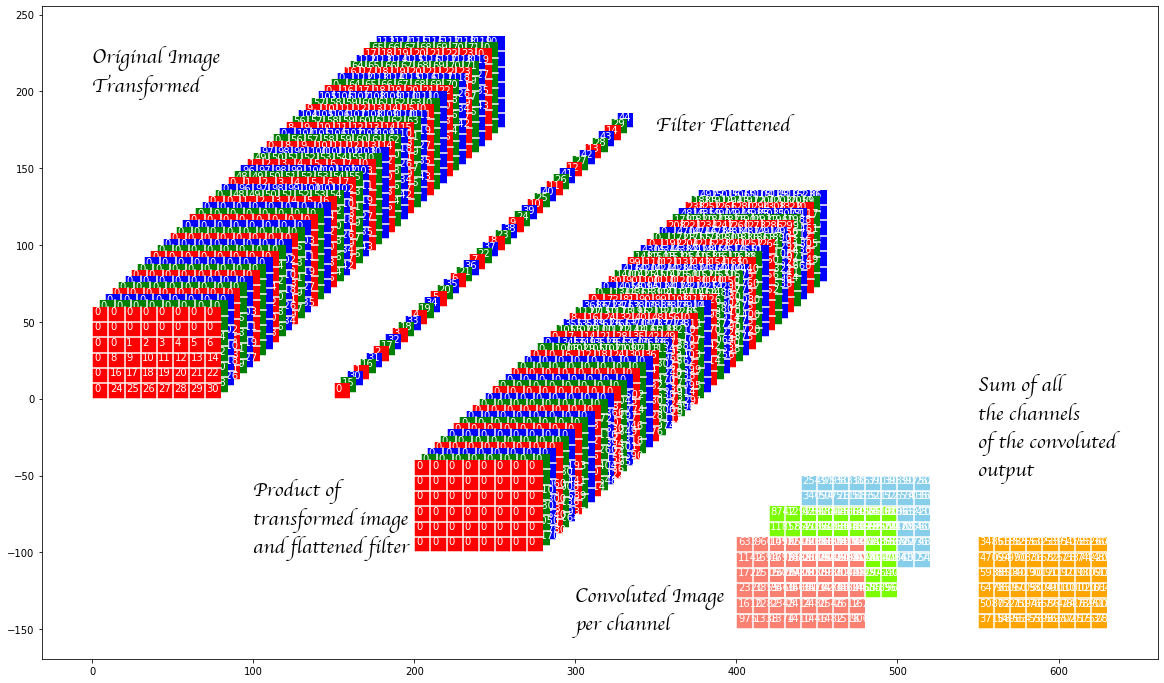
The procedure to obtained \(\bar l^0\) from \(\tilde l^0\) is straightforward and is best explained by the code that is given below. However, let us first visualize what is happening.

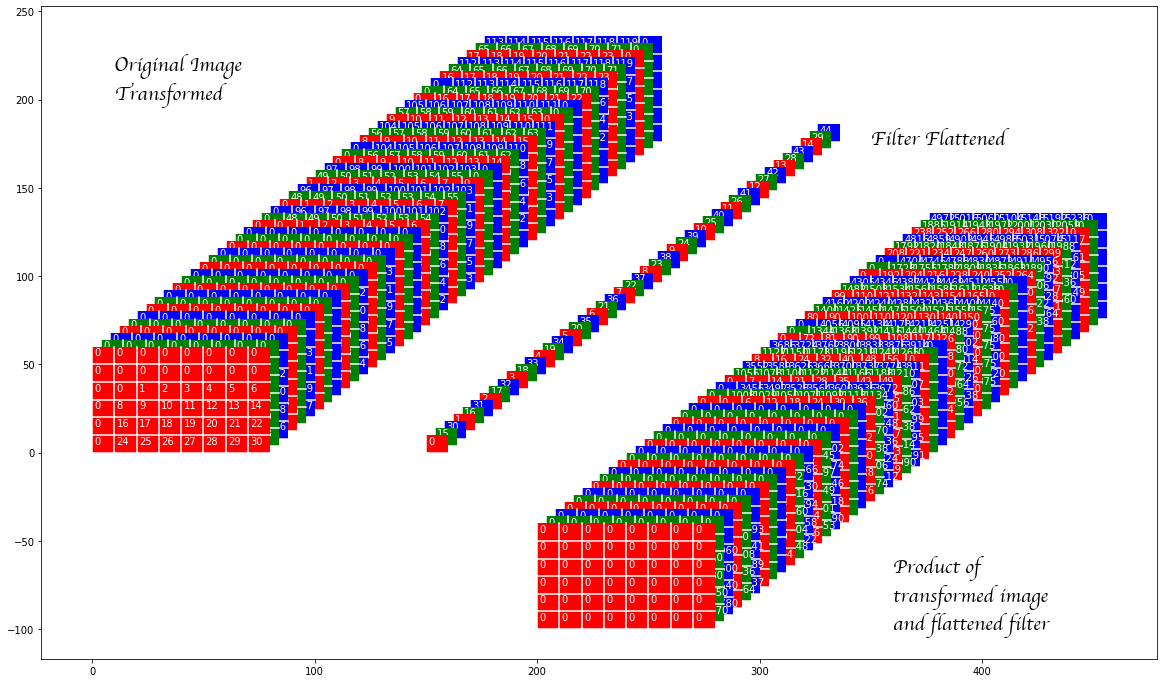
In the image above the original image transformed consists of the elements of the zero padded image rearranged (with duplication) so that each panel (the panels are laid out in the depth direction) contains all the elements that are to be multiplied by on element of the convolution filter. The convolution filter itself is raveled out in the depth direction (and we refer to it as the flattened filter in the image above).  The product of these two are shown next.

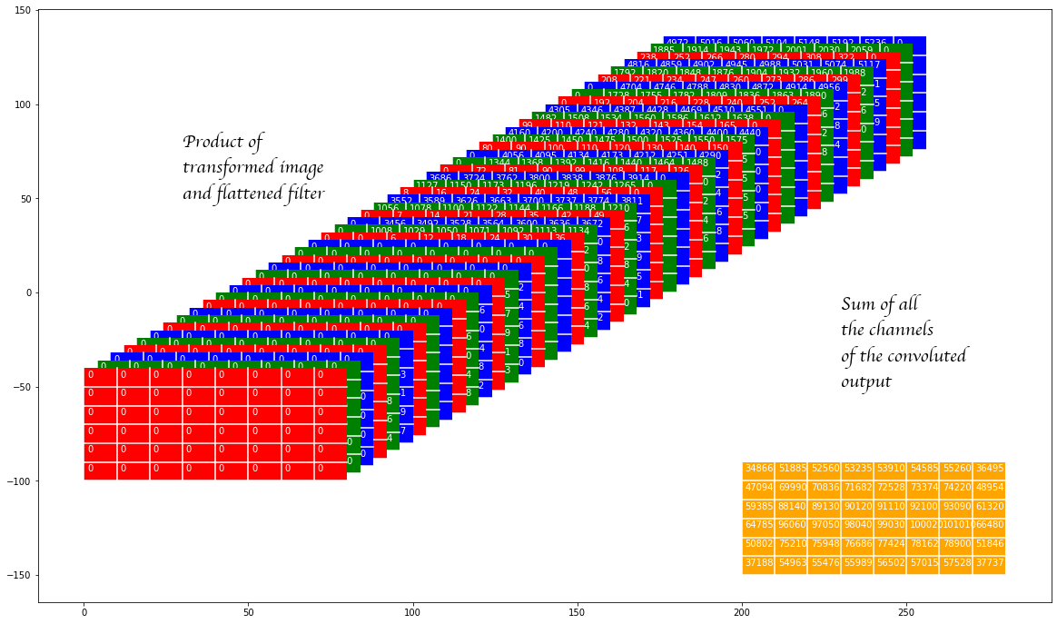
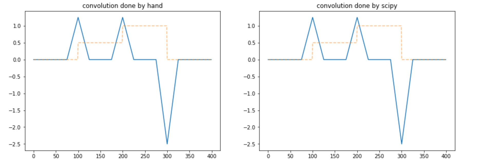
The product of transformed image and the flattened filter is shown again and then we show the sum of all these panels. One can verify that the results are the same.

The code to get the aforementioned transformed image from the zero padded image is given below and this is the main point of this post. Again, the code is part of the CNN layer and hence the reference to ‘self’ but the the meaning should be clear.

def _take(self, y, stride=(1, 1)):

    stride_1, stride_2 = stride
    mb, en1, en2, ch = y.shape

    # Till we discuss the minibatch index, all comments are for the first
    # image

    # Make a 2d array of indices of the top-left edges of the windows
    # from which to take elements. These are to be the indices on the
    # first channel. This makes the indices the top-left-back end of the
    # cuboid to be taken
    s1 = np.arange(0, en1 - self.filter_size_1 + 1, stride_1)
    s2 = np.arange(0, en2 - self.filter_size_2 + 1, stride_2)
    start_idx = (s1[:, None] * en2 * ch + s2[None, :] * ch)

    # Make a grid of elements to be taken in the entire cuboid whose
    # top-left-back indices we have taken above. This is done only for
    # the first of the above cuboids in mind.
    # Note the cuboid elements are flattened and will now be along the
    # 4th direction of the output
    g1 = np.arange(self.filter_size_1)
    g2 = np.arange(self.filter_size_2)
    g3 = np.arange(ch)
    grid = (g1[:, None, None] * en2 * ch + g2[None, :, None] *
            ch + g3[None, None, :]).ravel()

    # Combine the above two to make a 3d array which corresponds to just
    # the first image in a minibatch.
    grid_to_take = start_idx[:, :, None] + grid[None, None, :]

    # Make and index for the starting entry in every image in a minibatch
    batch = np.array(range(0, mb)) * ch * en1 * en2

    # This is the final result
    res = y.take(batch[:, None, None, None] + grid_to_take[None, :, :, :])
    return res

The same code can be used in on the prepared \( \frac{\partial L}{\partial l^1}\) (see code above) to give a corresponding transformed version to perform the convolution for the backpropagation.

The remaining code is pretty straightforward and can be found in the repository mentioned at the beginning of the post.

Convolutional Neural Networks using Numpy – Part 1

There are many powerful tools like Keras and Tensorflow out there to make convolutional neural networks (CNNs). However, unless I have opened the hood and peeked inside, I am not really satisfied that I know something. If you are like me read on to see how to build CNNs from scratch using Numpy (and Scipy).

The code for this post is available in my repository

There are many powerful tools like Keras and Tensorflow out there to make convolutional neural networks (CNNs). However, unless I have opened the hood and peeked inside, I am not really satisfied that I know something. If you are like me read on to see how to build CNNs from scratch using Numpy (and Scipy).

I am making this post a multi part post. As of now I have planned two parts. In the first I will only do a two class classification problem on Fashion MNIST restricted to two classes. The images are monochromatic and the CNN will have only one convolutional filter followed by a dense layer. This simplicity will allow us to focus on the details of convolution without worrying about incidental complexity. In the second post I will tackle the full Fashion MNIST dataset (10 classes) and multiple convolution filters. I will also look at the CIFAR-10 dataset which has colored images in 10 classes.

This is going to a technical post and certain familiarity with algebra and calculus is assumed. While I know that one can do a lot with tensorflow without knowing advanced math, I do not see how it is possible to peek under the hood without the same. Algebra is essential in the forward pass and algebra and calculus are useful to compute the derivative of the loss function with respect to the weights of the network which I derive in closed form. These are used to update the weights, something commonly known as back propagation. Readers unwilling to go through the derivation but able to follow the final expressions can still benefit by understanding the final results and implementing (or following my implementation) in numpy.

Convolution

In this section we will discuss what exactly we mean by convolution in image processing and how it is related to the implementation in scipy. This is useful as scipy implementation is much faster than a naive numpy implementation. In the end we will consider an example where we compute the convolution by hand and by using scipy as a sanity check. For simplicity we will work in 1 dimension for this section but the arguments extend simply to any number of dimensions.

Mathematically a convolution of a function f by a function g is defined as

This definition is useful in physics and signal processing. For instance in electromagnetism g could be the charge density and f (called a Green’s function in that case) would help us compute the potential due to said charge distribution. (See books on electromagnetism like Jackson or particle physics like Peskin and Schroeder for more details).

In image processing this definition is a bit backwards in that for a convolution window g , of length , we would want the convolution at to be the weighted average of such that the value at −/2+ is weighted by (). Thus, for image processing purposes the correct definition is

Note that this will require value of f(x) for negative values of x and if this is put in as it is then numpy will interpret the negative numbers as indexing from the end of the array. Thus, while implementing this in numpy, we need to make sure that the original array is embedded in a bigger 0-padded one and negative indexes are understood appropriately.

In our implementation of CNNs, we will use scipy.convolve as it will be faster than a naive implementation in numpy. So it is useful to understand the way scipy.convolve is related to what we want. Scipy’s convolve is for signal processing so it resembles the conventional physics definition but because of numpy convention of starting an array location as 0, the center of the window of g is not at 0 but at K/2. So scipy.convolve uses the definition

Now, we if reverse the scipy convolution window we have y ->K-y and that makes the integral

Thus we will get the result we want by giving the reversed array of the convolution window to scipy.convolve.

As an example consider the signal and filter given below.

We then implement the convolution by hand and using scipy in the following command

convolve(sig,win[::-1],'same')

The results are plotted below. The reader is advised to convince herself that the results are the same either by eyeballing the graphs or implementing the two methods herself.

We are now ready to implement CNNs using numpy.

Two-class classification

As our first example we implement a two class classification using numpy. I discuss this in full detail and for the other examples in latter posts I will expect that the reader has understood this example in detail and go a bit faster.

For the data we will used the Fashion MNIST. We get this from Keras as it is easily available but do note that this is the only use of Keras in this post.

(X_train_full, y_train_full), (X_test, y_test) = keras.datasets.fashion_mnist.load_data()

We then restrict our dataset to just the category 1 and 3.

cond=np.any([y_train_full==1,y_train_full==3],0)X_train_full=X_train_full[cond]
y_train_full=y_train_full[cond]
X_test=X_test[np.any([y_test==1,y_test==3],0)]
y_test=y_test[np.any([y_test==1,y_test==3],0)]y_train_full=(y_train_full==3).astype(int)
y_test=(y_test==3).astype(int)

We then split our training set into a train and validation set

X_train, X_valid = X_train_full[:-1000], X_train_full[-1000:]
y_train, y_valid = y_train_full[:-1000], y_train_full[-1000:]

And we finally standardize the data as Neural Networks work best with data with vanishing mean and unit standard deviation.

X_mean = X_train.mean(axis=0, keepdims=True)
X_std = X_train.std(axis=0, keepdims=True) + 1e-7
X_train = (X_train - X_mean) / X_std
X_valid = (X_valid - X_mean) / X_std
X_test = (X_test - X_mean) / X_std

Our data are monochrome images that come as matrices of dimension L x L (here L=28). For simplicity we have only one convolution layer (we will relax this restriction in later posts) which is a matrix of size K x K (we will take K=3 in our examples) whose weights can be learnt. In addition we have a dense layer which is a matrix of size (L*L) x 1. Note that we have not kept bias terms and the reader can include them as an exercise once she has understood this example.

We now describe the forward pass, the error and the back propagation in some detail.

Forward Pass

  • We get the images and refer to it as the 0-th layer 0
  • We embed the image centered into one of size (+,+) with zero padding
  • Then we pass it through a convolutional layer and an activation function f1 (that we will take to be Relu). This is the first layer l1.
  • Finally we make a dense layer wrapped in a function f2 (which in this case we take to be a sigmoid function). This is the second layer l2.

Note that even though the weights W2 are for a dense layer we have written the indices here without flattening as it has an intuitive interpretation in that it takes each pixel of the convoluted image and makes a weighted sum. Nevertheless, flattening both and doing a numpy dot is more performant and that is what we do in the code below.

For the loss function we take the usual log-loss

where y is the true outcome.

Backpropagation is just a fancy word for saying that all the learnable weights are corrected by the gradient of the loss function with respect to the weights that are being learned. It is straightforward to differentiate the loss function with respect to W1 and W2 using the chain rule.

  • The derivative of the loss function with respect to the layer 2 is

  • The derivative of the loss function with respect to the dense layer weights is

where we have used the fact that l2 is the output of the sigmoid function s(x) and that s’(x)=s(x)(1-s(x)).

  • Similarly, the derivative of the loss function with respect to layer 1 is

  • The derivative of the loss function with respect to the convolution filter is

Now we have closed form expressions for the derivative of the loss function with respect to the weights of the convolution filter as well as the final dense matrix so we can update the weights (with a hyperparameter the learning rate) as

That’s it.

That is all that is required to write the implementation of the CNN. Before doing that we first note the loss function and accuracy for initial random weights so as to have a benchmark.

Before training starts, the loss on average can be obtained analytically from the expression for the loss and is 1. The accuracy is 0.5. We will run our code over five epochs and see the loss and accuracy on the test and validation set.

First we write some custom functions for Relu, its derivative and the sigmoid function that we require for the main code and a function to just do the forward pass and compute loss and accuracy to do so on the validation set

def relu(x):
    return np.where(x>0,x,0)
    
def relu_prime(x):
    return np.where(x>0,1,0)

def sigmoid(x):
    return 1./(1.+np.exp(-x))

def forward_pass(W1,W2,X,y):
    l0=X
    l0_conv=convolve(l0,W1[::-1,::-1],'same','direct')    

    l1=relu(l0_conv)    
    l2=sigmoid(np.dot(l1.reshape(-1,),W2))
    l2=l2.clip(10**-16,1-10**-16)    
    loss=-(y*np.log(l2)+(1-y)*np.log(1-l2))
    accuracy=int(y==np.where(l2>0.5,1,0))    
    return accuracy,loss

Now we write the main part of the code

# learning rate
eta=.001
for epoch in range(5):    
    # custom code to keep track of quantities to 
    # keep a running average. it is not shown for clarity. 
    # the reader can implement her own or ask me in the comments.    train_loss, train accuracy=averager(), averager()
    
    for i in range(len(y_train)):
        
        # Take a random sample from train set
        k=np.random.randint(len(y_train))
        X=X_train[k]
        y=y_train[k]

        ##### FORWARD PASS ######        
        
        # First layer is just the input
        l0=X
        
        # Embed the image in a bigger image. 
        # It would be useful in computing corrections 
        # to the convolution filter        
        lt0=np.zeros((l0.shape[0]+K-1,l0.shape[1]+K-1))
        lt0[K//2:-K//2+1,K//2:-K//2+1]=l0
        
        # convolve with the filter
        # Layer one is Relu applied on the convolution                l0_conv=convolve(l0,W1[::-1,::-1],'same','direct')
        l1=relu(l0_conv)        

        # Compute layer 2
        l2=sigmoid(np.dot(l1.reshape(-1,),W2))
        l2=l2.clip(10**-16,1-10**-16)
        
        ####### LOSS AND ACCURACY #######
        loss=-(y*np.log(l2)+(1-y)*np.log(1-l2))
        accuracy=int(y==np.where(l2>0.5,1,0))
        
        # Save the loss and accuracy to a running averager
        train_loss.send(loss)
        train_accuracy.send(accuracy)        

        ##### BACKPROPAGATION #######
        
        # Derivative of loss wrt the dense layer
        dW2=(((1-y)*l2-y*(1-l2))*l1).reshape(-1,)
        
        # Derivative of loss wrt the output of the first layer
        dl1=(((1-y)*l2-y*(1-l2))*W2).reshape(28,28)
        
        # Derivative of the loss wrt the convolution filter        f1p=relu_prime(l0_conv)
        dl1_f1p=dl1*f1p
        dW1=np.array([[
           (lt0[alpha:+alpha+image_size,beta:beta+image_size]\
           *dl1_f1p).sum() for beta in range(K)]\
           for alpha in range(K)])  
      
        W2+=-eta*dW2
        W1+=-eta*dW1    
    loss_averager_valid=averager()
    accuracy_averager_valid=averager()   
    
    for X,y in zip(X_valid,y_valid):
        accuracy,loss=forward_pass(W1,W2,X,y)
        loss_averager_valid.send(loss)
        accuracy_averager_valid.send(accuracy)
    
    train_loss,train_accuracy,valid_loss,valid_accuracy\
            =map(extract_averager_value,[train_loss,train_accuracy,
                 loss_averager_valid,accuracy_averager_valid])
    
    # code to print losses and accuracies suppressed for clarity

On my trial run I got the following results. Your’s should be similar

We can see that even this simple model reduces the loss from about 1 to 0.1 and increases the accuracy from 0.5 to about 0.96 (on the validation set).

We can visualize the convolution by plotting a few (standardized) images and their convolution with the original random filter and the final trained one.

Convolution of image 1 using the initial random filter and the final learned filter

Convolution of image 2 using the initial random filter and the final learned filter

Convolution of image 3 using the initial random filter and the final learned filter

We see that the convolution filter seems to have learned to identify the right edges somewhat. It should be better when we train multiple filters but we have kept things simple by having just one filter. (This choice itself is a hyperparameter). We can do one more thing before finishing off part 1 of this post. We can make two more models: 1) We freeze the convolution layer weights and 2) We freeze the dense layer weights. This would help us understand if these layers contribute to the process. This is very easy. For the former we comment out the update line for W1

W2+=-eta*dW2
# W1+=-eta*dW1

and for the latter we comment out the update line for W2

# W2+=-eta*dW2
W1+=-eta*dW1

The resulting loss and accuracy are

and

respectively. It is clear that most of the work is done by the dense layer but we can still get a loss of .5 and an accuracy of .8 by just the convolution layer. Presumably this performance will increase with a larger number of filters. We will explore this in later posts.

Machine Learning and Knowledge Management

Last Friday, I had the opportunity to present to the DC Chapter of the Knowledge Management Association. I went over different ways artificial intelligence can be applied to help address challenges facing knowledge management. It was a great experience and I learned a lot from the questions and interactions with our local KM experts. Here are the slides: KMA Presentation

Creating Centaurs

The promise of artificial intelligence is to teach computers to understand the world so they become better at helping us interact with it.

In 1997, the artificially intelligent machine Deep Blue defeated the reigning chess champion, Garry Kasparov. Its victory didn’t spell the end of the human endeavour of chess; rather, it heralded in a new era of human-machine synergy. Today’s best chess players are “Centaurs” – human chess experts enhanced and backed by the power of artificial intelligence. Continue reading “Creating Centaurs”